Divvy, Chicago's iconic bike share system is about to pass the 10 million trip mark!

As bike shares proliferate across the U.S., the success of Divvy (the largest system by number and coverage of stations) has inspired other cities to invest in their own bicycle infrastructure. Users can purchase an annual membership (at a discounted rate for low-income residents), or a 24-hour pass to use the bicycles. Bikes may be picked up at any station and dropped off at any other station in the network.

Trip data

As part of Chicago's Open Data initiative, the Divvy trip dataset is publicly available and updated quarterly. The dataset can be queried through the Socrata Open Data API (SODA). The package sodapy provides a Python interface to SODA.

:::python
%matplotlib inline
import sodapy
import matplotlib.pyplot as pp
import numpy as np
import smopy

data_url = 'data.cityofchicago.org'
divvy_data = 'fg6s-gzvg'

Each dataset row is a single station-to-station bike trip including start and stop time, station information, and whether or not the rider was a member or a 24-hour pass user (gender and birth year is provided if the user is a member). Any given bicycle may diffuse throughout the network in a series of trips. A typical series of 10 trips is shown below:

:::python
# Get most recent 10 trips
data = sodapy.Socrata(data_url, None)
trip_chain = data.get(divvy_data, bike_id=2538,
                      limit=10, order='stop_time ASC')
data.close()

map_chi = smopy.Map((41.86, -87.645, 41.93, -87.605), z=14)
ax = map_chi.show_mpl(figsize=(8, 6))

for t in trip_chain:
    print t['from_station_name'], ' >> ', t['to_station_name']

    from_lat = float(t['from_latitude'])
    to_lat = float(t['to_latitude'])
    from_lon = float(t['from_longitude'])
    to_lon = float(t['to_longitude'])

    x1, y1 = map_chi.to_pixels(from_lat, from_lon)
    x2, y2 = map_chi.to_pixels(to_lat, to_lon)

    ax.plot([x1, x2], [y1, y2], 'r')
    ax.plot(x1, y1, 'go')
    ax.plot(x2, y2, 'r*')

pp.show()

Stetson Ave & South Water St  >>  McClurg Ct & Illinois St
McClurg Ct & Illinois St  >>  Michigan Ave & Oak St
Michigan Ave & Oak St  >>  Theater on the Lake
Canal St & Madison St  >>  Michigan Ave & Lake St
Millennium Park  >>  Adler Planetarium
Adler Planetarium  >>  Fairbanks Ct & Grand Ave
Clinton St & Washington Blvd  >>  Wells St & Erie St
Wells St & Erie St  >>  Clinton St & Washington Blvd
Canal St & Adams St  >>  State St & Erie St
State St & Erie St  >>  Dearborn St & Adams St

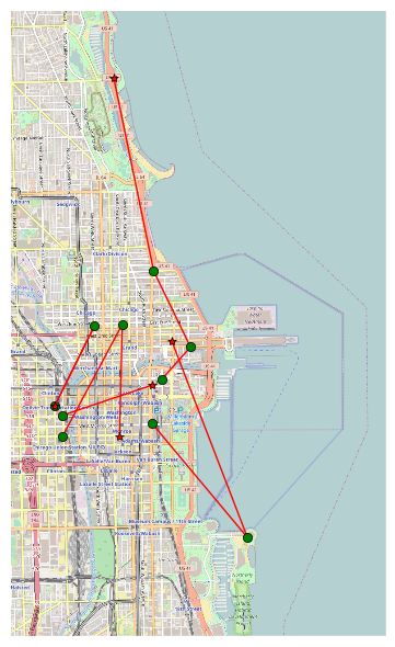
Notice that some trips are contiguous (begin at the station where the last trip left off), while others are not. Divvy removes bikes from stations for load-balancing, maintenance, and special events (like the Divvy triathalon). Unless the bike is returned to the same station (unlikely), there is a break in the chain of trips.

Analyzing trip chains

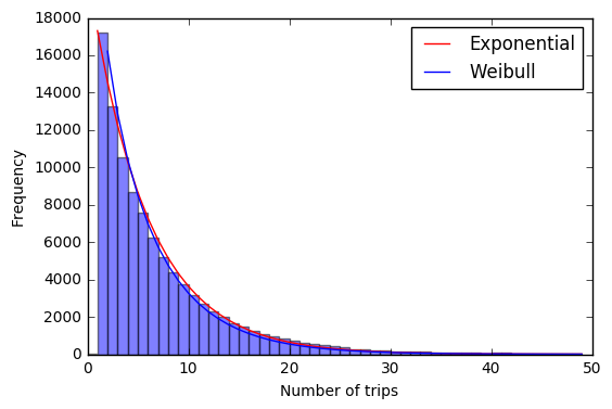
By querying all trips (yes all 10 million of them!) and organizing them into contiguous trip chains, we can get some insight into how and how frequently Divvy removes bicycles. Using a separate script, I analyzed each trip chain and recorded the bike ID, the number of trips in the chain, and the start and end stations. The script below loads the tripchains data, generates a histogram of trip chain length, and fits two different distributions to the data.

:::python
import scipy.stats
n_tc = 100000      # Number of tripchains to include in average
tc_len = [0]*n_tc  # Tripchain length

with open('tripchains.txt') as f:
    f.readline()  # Discard header row
    for i in range(n_tc):
        line = f.readline().split(',')
        tc_len[i] = int(line[1])

# Average statistics
print 'Average tripchain length: {:4.2f}'.format(np.mean(tc_len))

# Fit exponential distribution
# exponential statistics would be expected if bike removal is a Poisson process
exp_loc, exp_scale = scipy.stats.expon.fit(tc_len)
exp_dist = scipy.stats.expon(loc=exp_loc, scale=exp_scale)

# Fit Weibull distribution
wei_c, wei_loc, wei_scale = scipy.stats.dweibull.fit(tc_len, floc=1.0)
wei_dist = scipy.stats.dweibull(c=wei_c, loc=wei_loc, scale=wei_scale)
print 'Weibull shape factor: ', wei_c

# Truncate histogram to 50 trips
pp.hist(tc_len, bins=range(50), alpha=0.5)
pp.plot(bins[1:], n_tc*exp_dist.pdf(bins[1:]), 'r', label='Exponential')
pp.plot(bins[1:], 2*n_tc*wei_dist.pdf(bins[1:]), 'b', label='Weibull')

pp.xlabel('Number of trips')
pp.ylabel('Frequency')
pp.legend()
pp.show()

Statistics of bike removal

If bikes are removed completely randomly (from the bike's perspective, not necessarily the station's), then we would expect trip chains to approximate a Poisson process (I analyzed the video game Super Hexagon as a Poisson Process in a previous post). Indeed, the exponential distribution fits the data very well and gives an average trip chain length of 6.78 trips. The cumulative distribution function for the exponential distribution is

where \(x\) is the trip length. An important consequence of the exponential distribution is that the probability of a bike being removed in any given time interval is constant.

On the other hand, if bikes were removed mainly for maintenance purposes, we would probably expect that bikes which have been in the system longer would have a higher probability of needing routine maintenance, so the probability of removal would increase with time. If the probability of removal follows a power law with time, then the trip length could be approximated with a Weibull distribution.

The shape factor, \(c\), tells us how the probability changes with time. If \(c=1\), then the probability of removal is constant and the Weibull distribution is identical to the exponential distribution. The shape factor approximated from the data is \(c=0.95\), which is not significantly different from 1. So it's likely that either - most Divvys are pulled for load balancing or special events and they are chosen at random, or - most mechanical failures are related to random occurances like flat tires, crashes, or vandalism rather than component wear.

My code is available on GitHub. The map is from OpenStreetMap.